Notes for CS229 - Lecture 3

Notes based on CS229 Lecture 3

These notes cover the classification problem. For now, we will focus on the binary classification problem, in which $y$ can take on only two values, 0 and 1. His example use case of classification was classifying tumours as benign or malignant, as I work in cancer research this was particularly motivating.

Table of contents

Logistic Regression

For binary classification, we now want our hypothesis to output values 0 and 1, i.e. $h_{\theta}(x) \in \{0, 1\}$

So we will replace the hypothesis function as follows: $h_{\theta}(x) = g(\theta^{T}x) = \frac{1}{1+e^{-\theta^{T}x}}$

$g(z) = \frac{1}{1+e^{-z}}$, this is called the “sigmoid” or “logistic function”.

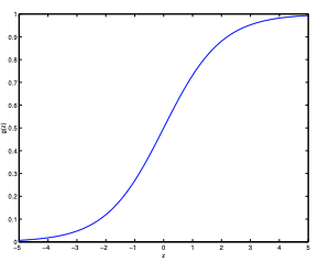The graph shows asymptotes at 0 and 1.

It will take $\theta^{T}x$ and pass it through the sigmoid function, so it’s forced to output values only between 0 or 1.

This is a common theme, for a new learning algorithm we will choose a new $h(\theta)$.

Now, let us assume that:

$P(y=1 | x; \theta) = h_{\theta}(x)$ $P(y=0 | x; \theta) = 1 - h_{\theta}(x)$

We then establish the probability density function, define the log likelihood, and perform Maximum Likelihood Estimation (MLE) (see full working out in lecture notes for this) we are then left with a formula we want to maximise.

If we use gradient ascent defined by:

$\theta := \theta + {\alpha}\triangledown_{\theta}\ell(\theta)$

And subtitute in the partial derivative of $\ell(\theta)$, we are left with:

$\theta_j := \theta_j + \alpha(y^{(i)} - h_{\theta}(x^{(i)}))x_{j}^{(i)}$

This therefore gives us the stochastic gradient ascent rule.

If we compare this to the least means squares update rule, we see that it looks identical, but this is not the same algorithm, because $h_{\theta}(x^{(i)})$ is now defined as a non-linear function of $\theta^{T}x^{i}$.

It’s surprising we end up with the same update rule for a different algorithm and learning problem. There is a deeper reason behind this, answered in the GLM models next lecture.

Newton’s method

Gradient ascent takes quite a few iterations to find the maximum. Newton’s method lets us take much bigger leaps (with the disadvantage that each iteration will be much more computationally expensive.)

The generalization of Newton’s method is given by:

$\theta := \theta - H^{-1}\triangledown_{\theta}\ell(\theta)$.

Where $H$ is a $d+1-by-d+1$ matrix (assuming that we include the intercept term) named the Hessian, the entries of which are given by:

$H_{ij} = \frac{\partial^{2}\ell(\theta)}{\partial\theta_{i}\partial\theta_{j}}$

Newton’s method typically enjoys faster convergence than (batch) gradient descent, and requires many fewer iterations to get very close to the minimum. One iteration of Newton’s can, however, be more expensive than one iteration of gradient descent, since it requires finding and inverting an d-by-d Hessian; but so long as d is not too large, it is usually much faster overall.